Why you shouldn’t take your data at face value — and what Inferential Statistics can do about it

The line goes up, so it must be working. The line goes down, so it’s not. Right? Not necessarily. Treating every visible trend as hard proof is one of the most common and most costly mistakes I see in data-driven organisations.
I recently gave an internal seminar at Wimmy on inferential statistics, and I want to share some of the core ideas here, because whether you run a hospital, a health insurance company, or a MedTech organisation, these ideas can save you from expensive wrong conclusions.
Three branches of statistics, one blind spot
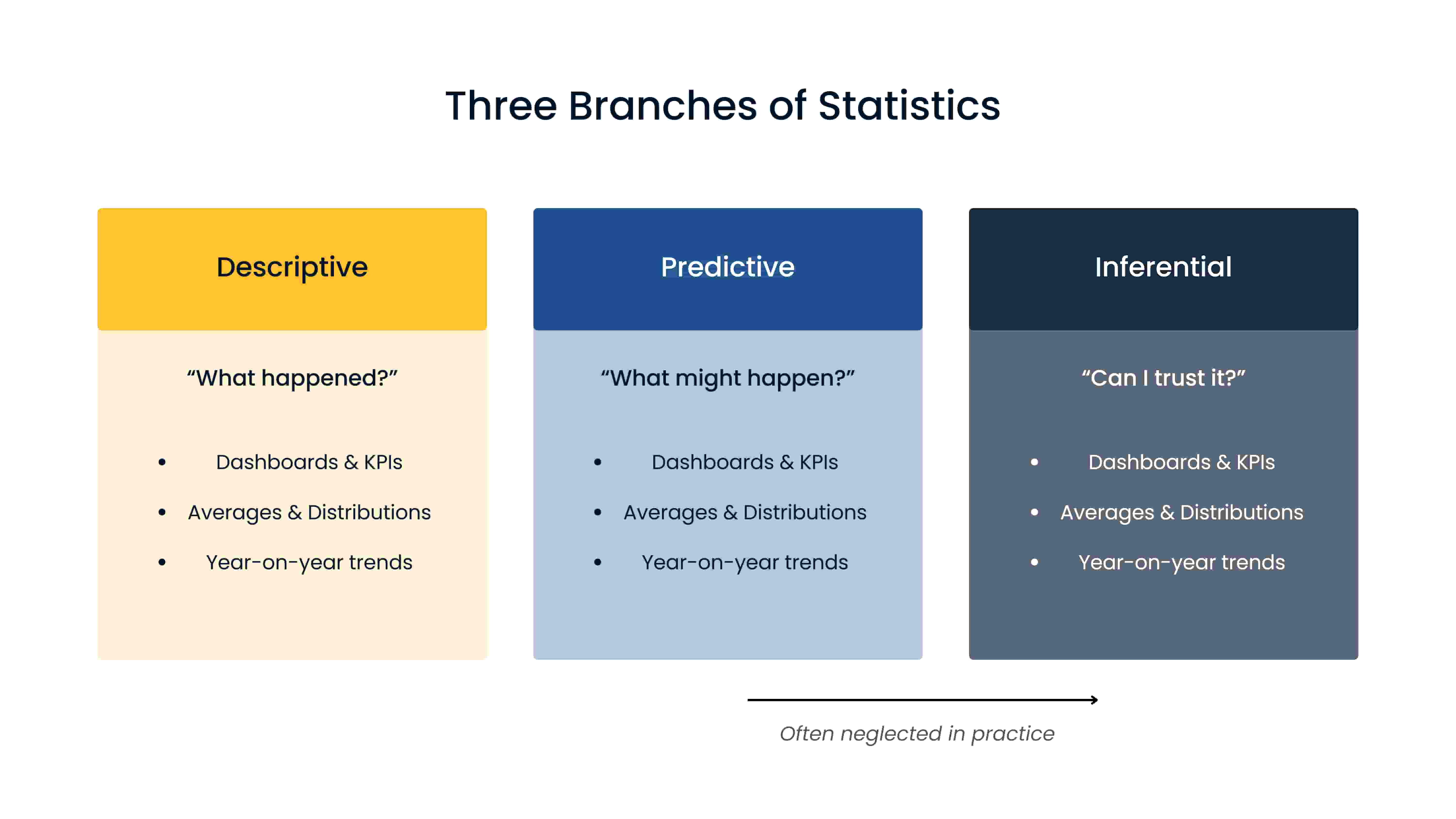
Most people think of statistics as a single discipline. In practice, it breaks into three branches, each answering a different question.
Descriptive statistics answers “what happened?” This is your dashboards, your KPIs, your year-on-year trends. If a client asks “how many patients did we see last year, and has that number been going up or down?”, five data points and a trend line answer the question. No p-values required.
Predictive statistics answers “what might happen next?” Think machine learning models, demand forecasting, or risk scoring. A typical example is predicting whether a patient is likely to miss their appointment, based on their characteristics.
Inferential statistics answers a fundamentally different question: “can I trust what I’m seeing?”
In my experience, the vast majority of analytics work in non-academic organisations is descriptive. Predictive statistics have grown enormously thanks to machine learning. But inferential statistics are often the most neglected. And that can have dangerous consequences.
It all starts with variation
Inferential statistics is built on two foundational observations.
The first is that everything varies. No two patients, students, transactions, or consultations are identical. Heights differ, weights differ, error rates differ. If nothing varied, we wouldn’t need statistics at all.
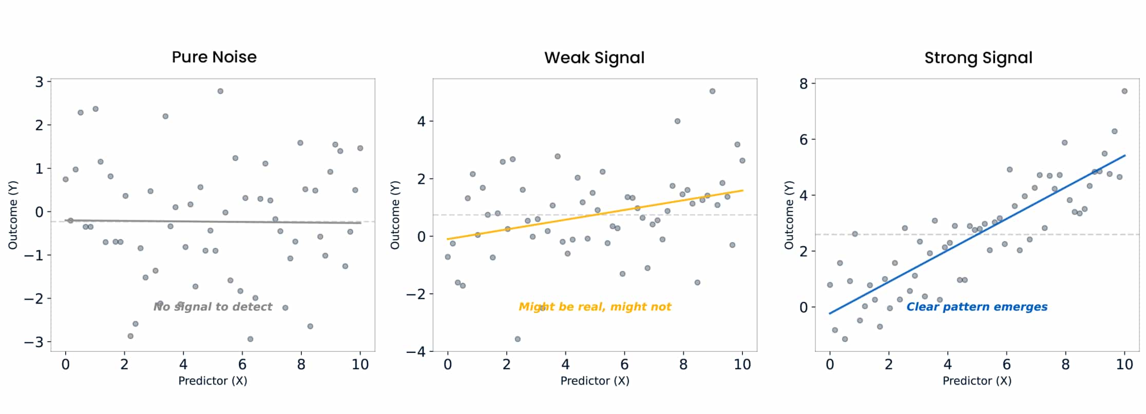
The second is that not all of that variation is random. Some of it is explained by age, gender, treatment, time, geography, or any number of other factors. If I know your age, I can make a better estimate of your weight than if I know nothing about you. That improvement in estimation over pure guessing is the signal we’re trying to detect.
If there were no variation, statistics would be unnecessary. If all variation were random, we’d stop at descriptive statistics. We’d report the average, draw the histogram, and move on. Inferential statistics enters the picture when we have a hypothesis about what explains the variation and we want to test whether the data supports it.
The null hypothesis: your built-in sceptic
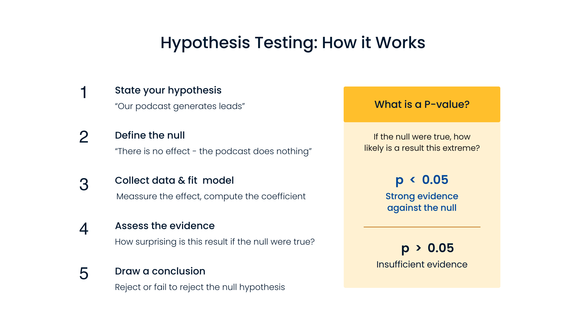
Here’s the basic mechanics. You start with a hypothesis. For instance, “our podcast marketing is generating new leads.” Then you define the null hypothesis: the default position that there is no effect. The podcast does nothing. The null is your built-in sceptic. It says: “Prove me wrong.”
You collect data, fit a model - perhaps a simple regression model - and look at the coefficient. That coefficient is never going to be exactly zero. There will always be some observed difference. The question is whether that difference is large enough to make “random variation by chance” an implausible explanation for the difference.
This is what a p-value quantifies. If the null hypothesis were true, i.e. if there really were no effect, a p-value of 0.02 means there’s only a 2% probability of observing a test statistic (= a special summary statistic of the data) as far or further removed from the one you’d expect under the null hypothesis as the one you got. A very small p-value indicates it’s highly unlikely to observe the data you have in a world where the null hypothesis is true.
One important nuance: a p-value does not tell you the probability that your hypothesis is true, and it does not tell you how often future studies would replicate your result. It speaks only to how surprising your data would be under the assumption of the null hypothesis.
Confidence intervals: the honesty check
Where p-values give you a single signal of “statistical significance, confidence intervals give you something richer: a range of plausible values for the true effect.
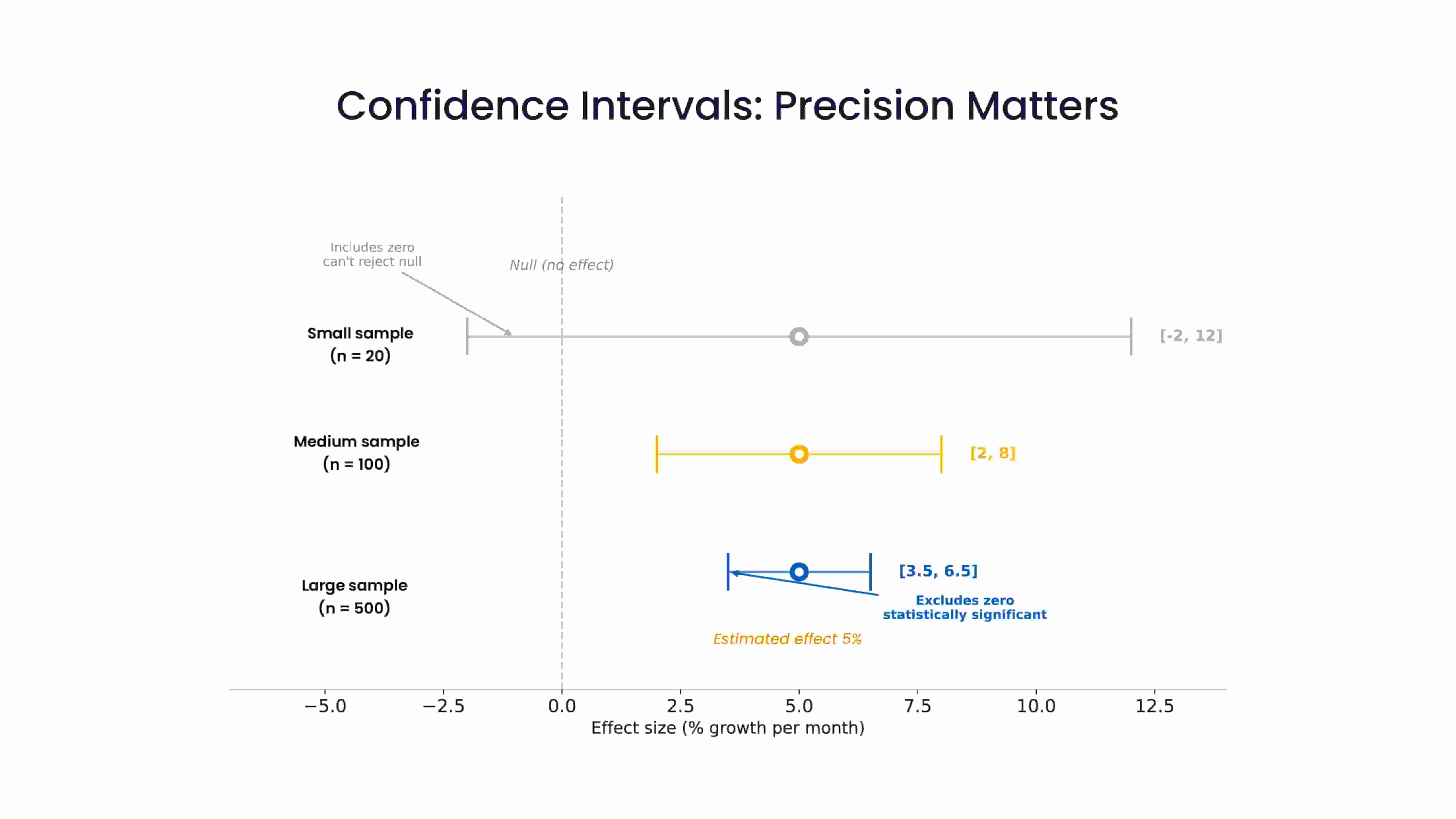
A wide interval tells you your data is consistent with many possible realities. In other words, you haven’t measured precisely enough. A narrow interval means you’re converging on an answer.
This is where inferential statistics can add very practical value. Instead of declaring “Clinic A’s utilisation rate grew by 5% per month” as if it’s a law of physics, you can say “we estimate 5% growth, with a 95% confidence interval of 1% to 9%.” Those are very different statements. The first invites overconfidence. The second invites better decisions. And if the 95% confidence interval spanned the range from -3% to 13%, that would indicate that it is not implausible that the growth was merely random noise, and that we should not be surprised to see stagnation or even shrinkage in the utilisation rate in the near future.
Sample size: how much data is enough?
A question that comes up in every project: how much data do we need? The answer depends on four things: the “power”, i.e. the probability your analysis will reject the null hypothesis if indeed the alternative hypothesis is true, the significance level, i.e. the probability that your analysis will incorrectly reject the null hypothesis when it is actually true (most often set at 5%), the amount of natural variation in your population, and the size of the effect you’re trying to detect.
If everyone within a group is nearly identical, you don’t need many observations to spot a difference between groups. If there’s enormous variation within each group, you need a much larger sample to separate signal from noise.
You can calculate the required sample size before collecting data, but you’ll need a prior estimate of the population’s variability, often derived from pilot data or previous studies. It’s a bit chicken-and-egg, but it’s a tractable problem.
Representativeness: who are you actually studying?
Sample size tells you how precisely you can measure an effect. Representativeness tells you how far you can generalise it.
If you sample 100 nurses from a single hospital, your findings might be representative of that hospital, but probably not of all private hospitals in the country, and certainly not of all nurses globally. The further you move from the specific context in which the data was collected, the shakier your conclusions become.
This isn’t a reason to avoid inference. It’s a reason to be transparent about its boundaries. Every study should state clearly: this is the population we sampled from, and this is as far as we’re comfortable generalising.
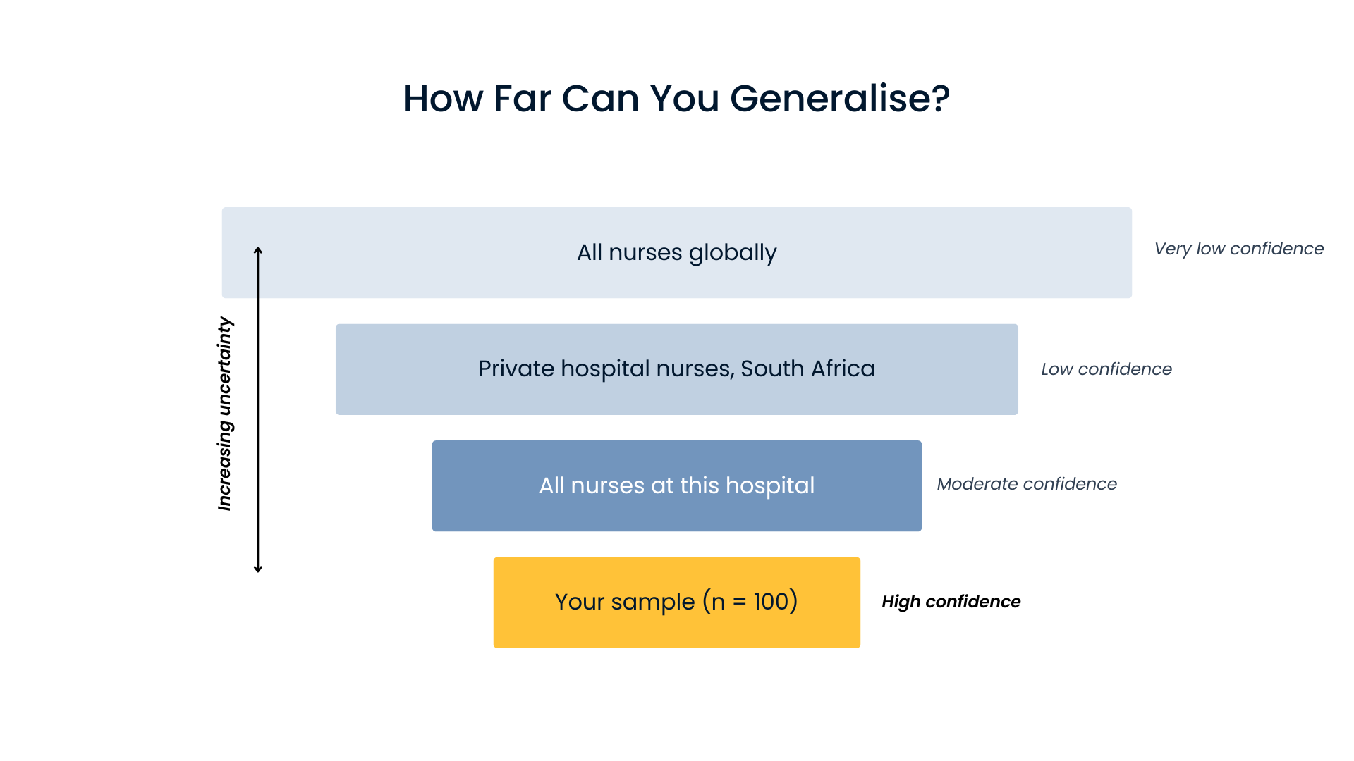
the weaker your conclusions become.
The practical trap: mistaking trends for truth
Here’s the scenario I’ve seen play out many times, and it’s the reason I think inferential statistics deserves more attention outside academia.
A company launches an initiative: a new campaign, a process change, a tool deployment. They look at the data after a few weeks. The trend line goes up. Success is declared, resources are committed, strategies are built on the finding.
But nobody asked the critical question: is this trend distinguishable from random noise?
Inferential statistics might have shown that the confidence interval around that slope was wide enough to be consistent with both “it’s working” and “it’s not working.” The honest answer was: we don’t have enough data yet. Keep collecting.
The reverse is equally dangerous. A promising initiative gets killed because the early data shows a dip, even though the dip falls well within the range of normal random variation. With a bit more patience and a confidence interval, the decision might have been very different.
A/B testing: inference in action
One of the clearest applications is A/B testing. You want to know whether a red website background outperforms a blue one. You expose some visitors to each version and compare click-through rates.
There will always be a difference in the numbers. The question is whether that difference is consistent with random variation between two identical treatments, or whether it reflects a genuine preference. Without a formal test and a confidence interval, you’re guessing. With them, you’re making an informed decision.
Despite its ubiquity in tech, many organisations still haven’t adopted A/B testing — or when they have, they stop at “red got more clicks” without asking whether the difference is statistically meaningful.
The bottom line
Inferential statistics isn’t about making things more complicated. It’s about being clear about what the data actually says, and what it doesn’t.
The next time someone shows you a trend line and draws a confident conclusion, ask two questions: what’s the confidence interval around the slope estimate? and what’s the null hypothesis we’re testing against? If they can’t answer, the conclusion might be premature.
You don’t need a statistics degree to apply these ideas. AI assistants can generate the code and run the models. But you do need to know the right questions to ask. And that starts with understanding variation, hypotheses, and the humility that comes from knowing your sample data is never the whole story.